The Solar-Stellar Spectrograph

[ Home | About | Tech Info & Data | Publications | References ]      [ Site by Jeffrey Hall | Research funded by NSF ]

Creating order maps

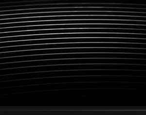
Fig. 1. A raw SSS flat field frame from the old (pre-2008) CCDs.

The image in Figure 1 at right is one of our raw flat field frames (flat for short). We take flats by shining white light through our optical faiber and into the spectrograph. This lets us record a white light spectrum that we use for two purposes. First, it creates a record of a perfectly "blank" star, which we use to calibrate and remove detector variations from the solar and stellar spectra. Second, it lets us create a map of where the spectral orders lie on the CCD. (Think of an "order" as "a chunk of spectrum." In technical terms, it's a diffraction order.) We need this map to locate the regions on the CCD where the spectrum falls, and extract only those parts for analysis. Thus, immediately after debiasing the data, we create an order map that is used in many of the subsequent reduction steps. An accurate map is important, since as you can see in Figure 1, only the blue Calcium HK spectral order at bottom is straight. All the other orders from the red spectrograph are curved (this is normal for a spectrograph such as ours). The software needs to be able to follow the curving orders to extract the data accurately.

Our three-pass method for order map creation

The Ordermap object of the OIL software creates an order map in three steps. The procedure is identical for the old and new cameras; the only difference is the number of orders (20 in the pre-2008 data, 16 afterwards).

Pass 1: Load and verify predetermined order locations

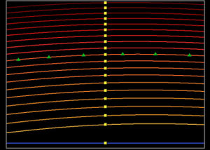
Fig. 2. A raw SSS flat field frame from the old (pre-2008) CCDs. Yellow squares are identified in the first step of ordermap creation. Green triangles show locations used for accurate order centroid calculation, and the full order traces (orange and blue lines) are determined in the third and final pass.

In small text files in the resource area of the SSS data archive, we store the pixel number along the y axis of the frame at which the order lies at the midpoint of the x axis. For our 512-pixel CCDs, this means pixel 256. The software loads the reference points (using different files for pre-2008 and 2008+ data) and checks to make sure the order peaks actually seem to be there. Yellow rectangles in Figure 2 show the result of this step.

Pass 2: Make crude order traces

The software then steps outward from the order midpoints, pixel by pixel, and finds the integer pixel where the maximum data value lies. This creates a crude, "jagged" trace of the orders.

Pass 3: Make an accurate final order determination

We then take six evenly spaced points along the order (shown for one order by the green triangles in Figure 2) and fit a Gaussian to the order profile across a 7-pixel wide aperture. The integer pixel values of the order peaks at those points are replaced by the floating-point Gaussian centroids. We then fit a second-order polynomial to the six triangles, and use the polynomial coefficients to determine accurate order peaks at every pixel along the dispersion direction for all the orders.

The result of all this for a typical pre-2008 flat is shown in Figure 2. The blue line is the Ca HK order. Since this is a single diffraction grating at third order, it is straight and almost perfectly aligned with row 16 on the CCD frame for both the old and new cameras. The echelle orders are shown by the yellow and red lines; they are second-order curves with order spacing increasing toward shorter wavelengths (toward the bottom of the frame), whuch is expected since the red spectrograph is a prism-cross-dispersed echelle. The method described above works extremely well for both the old and new cameras.

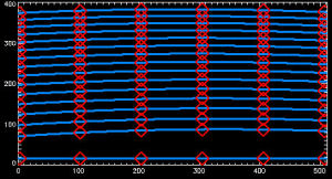
Fig. 3. The ordermap trace for the new (2008+) data.

"Old" versus "new" data

The effect of the 2008 camera switch for this step was negligble. We just needed to define a new reference file to identify the orders on the new CCD for the first order trace pass. We also had to generalize the software to know to look for only 16 orders in the post-2007 data rather than 20, but this likewise more tedious than difficult. Figure 3 shows a trace for the new data. We've adjusted the position of the six centroiding spots (red diamonds) to move them closer to the order ends, but this made no difference to the resulting maps.

Behavior of the order maps over time

Central order locations

We define a method of the OIL SSS class called SSS::ordermap_results. This method reads the diagnostic files created by the ordermap object and displays their contents. We first examine the overall location of the order map with time, i.e., the drift of the yellow squares in Figure 2 above over the entire data set. In Figure 4, we show the results for 1131 flat field frames taken between 1992 and 2009.

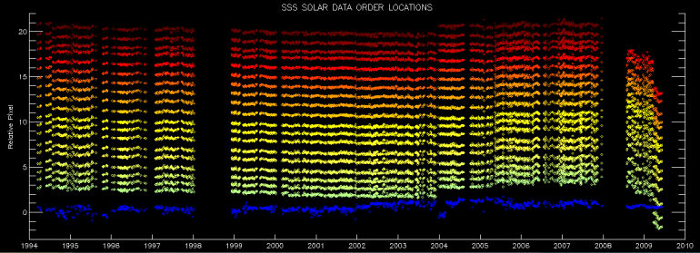
Fig. 4. The location of the order peak at the central pixel of each order for our solar data, 1992-2009. The gap in the data in 1998 corresponds to missing order maps resulting from our backup failure (causing loss of raw data only, not reduced spectra). The gap in 2008 results from the camera replacement, after which we extract only 16 orders rather than 20.

In this figure, the y-axis is an arbitrary pixel location; we have offset the actual order locations to fit them all conveniently on one plot and emphasize any drifts. The HK order (relative pixel 0) drifted within a range of ~ +/- 0.5 pixels over 14 years, with somewhat more scatter than is apparent in the echelle data (the 19 green to red colored orders). Of note is (1) a discontinuous jump of roughly 1 pixel in the echelle data at the start of 2004 and (2) a tendency for the new echelle camera to exhibit a systematic order drift of ~1 pixel between July and November 2008.

There is also a jump in the echelle order locations in early 2009. This corresponds to removal and replacement of the red CCD camera to repair a failed shutter. The order locations shifted by about 3 pixels (75 microns) after we replaced the CCD as precisely as possible.

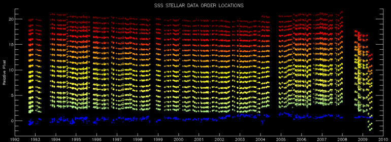
Fig. 5. The same plot as Figure 4, for the stellar data rather than the solar data, from 1992-2008.

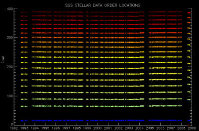
Fig. 6. Stellar order maps from 1994 to 2009, scaled to show the full 400-pixel range of the CCDs in the cross-dispersion direction.

In Figure 5 we show the order locations for our stellar flat field frames. The jump in order locations in 1994 is not surprising, because in late 1993 we began observations with new acquisition software that cropped the region of interest on the raw echelle frame slightly differently. We still see another order location jump in 2004, and a slow drift in the echelle locations for the new camera. The unexpected feature in this plot is the slight convergence of order locations immediately after the 2004 jump; the "green" orders drift upward by ~0.3-0.7 pixels, while the "red" orders remain relatively constant. This suggests a small change in the orientation or shape of the CCD, which in turn may affect the focus. Given the small magnitude of the drift, we do not expect this to be substantial.

Nevertheless, we will examine these drifts carefully in echelle data analysis to ensure no systematic effects stem from them. However, we also note that Figures 4 and 5 are scaled to significantly exaggerate the order map drifts over time. In Figure 6, we show the order locations scaled to show the full dimension of the raw frames in the cross-dispersion direction, with each order center plotted at its actual pixel rather than the arbitrary pixels of Figure 5. There is the known shift of the echelle orders after the 2008 camera replacement, but relative to our 9-pixel order apertures, the centroids have remained nearly constant over time, with an rms drift for all orders of < 0.1 pixel over 16 years.

Order profiles

As a final quality control check, we store the results of the Gaussian fits to the order profiles and ensure that valid fits are obtained for all points across the frame. A typical set of profiles appears in Figure 7.

Fig. 7. Each panel shows the six Gaussian fits to four of the orders in our data frames. The panel at left shows the six profiles for the HK order, while the three following panels show three of the orders from the echelle.

Each of the four panels in Figure 7 shows the Gaussian fits to the order profiles (i.e., the nine pixels across the order profile for the locations shown by red diamonds in Figure 3). Blue, green, and red lines indicate the fit points at the blueward (left), central, and redward (right) points for each order. Essentially, these figures show how the order profile changes as one looks down its dispersion axis.

For a "good" flat field frame, we should get valid fits at all six points for every order, since the peaks of the Gaussians above are used to define the polynomial coefficients that produce the final order map. This is the case for all flat field frames in the data base; we have discarded any flats for which profile fits fail. As you can see from Figure 7, the echelle fits in the three rightmost panels remain quite consistent. The defocusing of the HK order toward its ends is quite apparent (the very wide blue profiles in the leftmost panel). The focus is optimized and stable for the H and K region (the green fits near the center of the order).

  Continue to a description of flat fielding.  

[Back to contents]