The Solar-Stellar Spectrograph

[ Home | About | Tech Info & Data | Publications | References ]      [ Site by Jeffrey Hall | Research funded by NSF ]

Continuum normalization

Once we have extracted the spectra, there are just two steps left. We need to convert the x-axis of each spectral order from pixels to wavelength, and we need to normalize the continuum of the spectrum to unity. We discuss the latter step here. The spectrum is characterized by two components: the continuum, which is the generally smoothly varying spectrum of light emitted by the star, and the lines, which are the dark absorption features produced by particular atoms (or molecules) in particular atomic states. Here's the problem: suppose one exposure of a star has twice as many ADU as another. If we measured the amount of light in a given spectral line, we would erroneously conclude that in the first exposure, the star is twice as bright, which obviously can't be the case. The continuum, however, serves as a handy reference point, since for our purposes it is invariant. Therefore, we need to fit a smooth curve to the continuum in every spectral order, ande divide the spectrum by the fit. This set the continuum everywhere to 1.0, and allows us to measure the lines from spectrum to spectrum in a consistent way. It's very similar to how we normalize the flat field spectra. This procedure is a bit tricky, since picking out continuum points along each order is trivial for the human eye, but tougher to get a computer to do. The gory details are below.

Procedure

We normalize the continua of the spectra to unity as follows.

1. We first divide each order of the spectrum, including the Ca II H&K order, by the corresponding normalized blaze function stored during creation of the flat fields, using the flat field spectrum nearest in time to the target frame. This removes the most prounounced variations in the extracted continuum, rendering it nearly linear.

2. We have found by lengthy trial and error that the best way to fit the continuum for the echelle orders is to store a set of reference points for each order. We have a single reference point template for the solar spectra, and a set of files for stars of different spectral types. The normalization method loads the requested file and uses the predetermined points as a starting point for the fitting procedure. Generally we define 15-25 points for the various echelle orders. The Ca II H&K order is a different problem, since there is no well-defined continuum visible anywhere. For this order only, we use two pseudocontinuum points at 3912 and 4000 Å.

3. The normalizer object searches within +/- 5 pixels of each predetermined fit point to find the maximum spectrum value near the fit point. This is to allow for shifts of the spectrum due to instrumental effects (small) and radial velocity changes (large for some stars). This searches a velocity space of roughly +/-100 km/s, which is sufficient to account for nearly all Doppler shifts due to Earth motion and stellar radial velocities.

4. For the echelle orders, we fit a cubic spline to the grid of velocity-adjusted fit points, and divide the spectrum by the fit. For the Ca II H&K order, we fit a straight line to the two pseudocontinuum points, and divide the order by that fit.

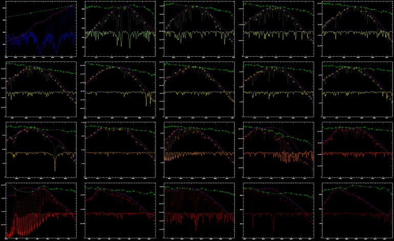
The result of all this is shown for all 20 orders of the old CCDs in Figure 1. Read on for a discussion, and some magnified images of part of this rather illegible figure.

Fig. 1. Here are all 20 orders of a typical solar frame. The HK order is at upper left, and the 19 echelle orders are arranged in rows in order of increasing wavelength. The spectra plotted across the middle of each panel are the normalized output; see below for discussion and details.

Discussion

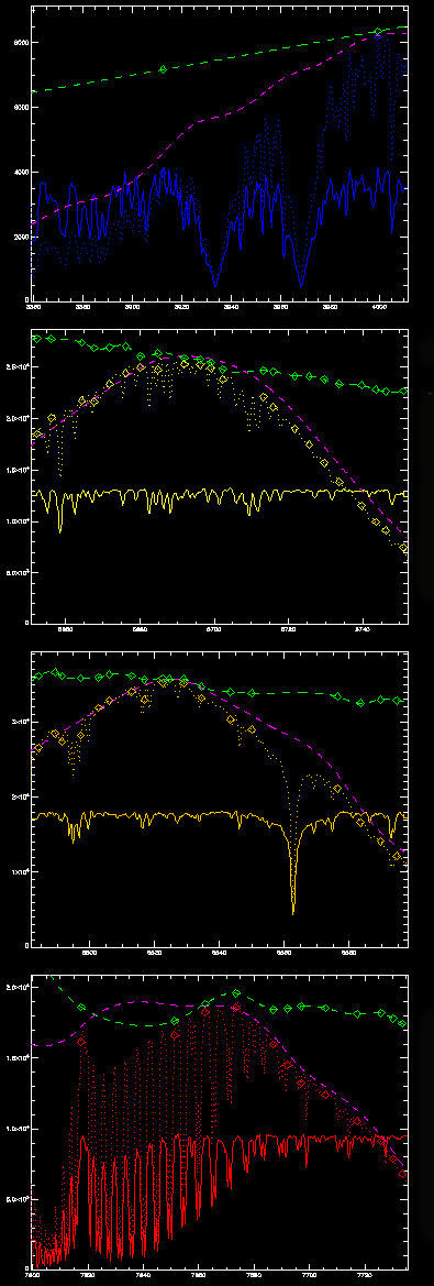
Fig. 2. This is a magnified plot of the first column of orders in Figure 1.

In Figure 2, we plot the first column of Figure 1, magnified so you can see what's going on. The top panel is Ca II H&K. The third panel contains Hα, and the bottom panel has the Fraunhofer A band of atmospheric oxygen.

The dotted lines show the non-normalized spectra (i.e., the output of the spectrum extraction. Their slanted or curving overall shape is the echelle blaze function. The solid plot in the same color (blue to red) is the final, normalized spectrum, divided by two for clarity on the plot.

We'll go back through each step of procedure listed above, referencing Figure 2.

1. When we divide by the blaze, which is shown by the dashed pink line, we theoretically should reduce each order to a linear continuum, with any slope simply resulting from the temperature difference between the flat field lamp and the order. This is apparent in the dashed green lines, which shows the final spline fit to the continuum points, and which also reflect this remaining color term closely. Clearly the lamp is hotter than the echelle and cooler than the HK order.

2 and 3. In each panel, you'll see diamonds of the same color as the dotted extracted spectrum. Those are the starting continuum reference points. Note how a few of them "fall" into the lines due to small velocity shifts. (Since this is the Sun, the problem is not severe, but with the stars, it can be much more so.) The green diamonds along each spline fit show the corrected fit points; i.e., the actual points used to make the fit. They now better reflect the true continuum.

4. The cubic spline fits to the points are shown by the green dashed line. In a world of perfect data, they should be straight lines. In the real world of Quasimodo-like data, they mostly look like the lines in the second and third panels. Panel 1 doesn't count, since the HK order is constrained to a first order polynomial fit. Panel 4 doesn't count because the A band is a perennial problem child, with no way to fit the nearly black bandhead at the blue end of the order. We don't lose sleep over this, since we don't use that part of the spectrum.

As we will show on some of the results pages, this normalization method produces continuum-normalized spectra with variations consistent with what we expect given the SNR of the data. Occasionally, however, there will be an unphysical dip or lump in an order or orders of a normalized spectrum. This arises from either of two circumstances: (1) the fit point shift fails to bring a fit point completely out of a line, causing the spline to dip and the normalized continuum to rise, and (2) a fit point finds a spike in the spectrum due to a readout glitch or cosmic ray hit, causing the spline to rise and the spectrum to dip.

We deal with these and any other pathological cases during the creation of the time series, as we will detail on other pages. Briefly, it is clear when a line measurement is discrepant due to a systematic offset in a spectrum, and we can either renormalize the spectrum to a properly normalized, "standard" spectrum of that star, or simply throw the data point away.

Occasionally, when we are so unfortunate as to have a large spike directly in the core of the Ca H or K line, we simply discard the observation. Our general philosophy is to discard bad data rather than try to "fix" them. This is a particularly easy philosophy to maintain when one can throw away the odd spectrum and still have a data set with the statistical weight of a brontosaurus!

One final detail: you may have noticed the Ca II H&K spectrum is not, in fact, correctly normalized. The 3912 and 4000 Å points are not true continuum but pseudocontinuum points. We need to scale the whole spectrum down so it lies accurately on an absolute intensity scale. This can be done quite reliably, and we detail it elsewhere.

[Back to contents]