The Solar-Stellar Spectrograph
[ Home | About | Tech Info & Data | Publications | References ] [ Site by Jeffrey Hall | Research funded by NSF ]
Removal of scattered light
The final task we must perform prior to extracting the spectral data is to remove any remaining scattered light that will introduce an artificial contribution to the spectra. We do this step immediately after the flat field division. The way we do this, described below, is to trace our way along the very edges of each spectral order and subtract the values we find at the edges from the entire order. This takes the order bases down to zero and yields a data frame ready for spectral extraction.
Procedure
We remove scattered light from the data frame in the following way.
1. For each order in the echelle frame, we trace the lower and upper boundaries of the curving order across the 512 pixels along the dispersion axis.
2. We determine the mean of the ADU values at the upper and lower order minima for each of the 512 pixels along the dispersion axis.
3. We fit a cubic spline to a grid of the mean ADU values at 50 evenly spaced points along the order.
4. We subtract the spline fit at each pixel along the dispersion axis from each pixel across the dispersion axis lying within the order apreture.
5. We use the same method on the HK order, but in a separate step since this order comes from a different CCD with only a single order and very low scattered light except at the red end of the order, where there is a noticeable increase in the background.
Description of the scattered light background
In Figure 1 below, we show the general results of the scattered light removal for a representative solar spectrum. This "dimetrodon plot" is a crosscut of the CCD frame through the orders along the midpoint of the dispersion axis. The ADU axis (y-axis) of the plot is scaled so that the low-level signals are visible; for this reason, the full range of the data goes well off the top of the plot.
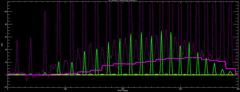
Fig. 1. A "dimetrodon plot" of one of our solar data frames. See text for description.
The tall, dotted purple spikes in Figure 1 are the raw, flat fielded data. The Ca HK order is at extreme left (pixels 1-32), and the echelle occupies the rest (pixels 33-400). Clearly visible between the main orders, which extend off the top of the plot, are ghost orders (in the echelle frame only). They look hideous, but their amplitude is small compared to the main orders.
The jagged pink line running across the plot is the scattered light background found for this point along the dispersion axis. Each order is treated as a separate strip of scattered light; this is a conscious decision in contrast to fitting a 2D polynomial to the entire echelle frame. The latter would produce a smoother surface, but the presence of the ghost orders occasionally obscures the order aperture minima and can lead to unphysical lumps in the 2D surface fit. We have found empirically that we obtain better fits to the order minima by treating the orders individually, and by determining scattered light values with a spline fit to a fairly dense set of points.
The outcome of the fit is shown by the solid green spectrum in Figure 1, which shows the "descattered" crosscut; the data values are also scaled down by a factor of 25 for visibility on the plot. The order bases are now nicely aligned at zero (solid yellow line), and the relatively small amplitude of the ghost orders is now more apparent.
Assessment of the procedure along the dispersion axis
It is instructive to examine plots of the scattered light fits along the dispersion axis, as well as in the cross-dispersion direction of Figure 1.
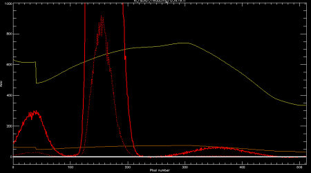
Fig. 2. The scattered light trace along a 512-pixel row of the echelle frame near the sodium D order.
In Figure 2, we show a trace of the scattered light spline fits along one row of the CCD. The data are in red, and the large humps are where the curving orders slice across the CCD row. (The main hump is the principal order, while the smaller ones are the nearby ghosts.) The dotted red line shows the data scaled down by a factor of 10.
The spline fit is shown in orange, and scaled up by a factor of 10 for visibility in yellow. The discontinuity in the fit at about pixel 40 is where the curving orders cause the CCD row to fall in different orders. I.e., the values from pixels 1 through 40 lie in aperture N, while the rest lie in aperture N+1.
As can be seen, the scattered light background ranges from about 34 at the red (right) end of the order to a maximum of about 75 near the order center. The peak ADU value in this order of this frame is about 9000, so the scattered light is less than 1% of the signal.
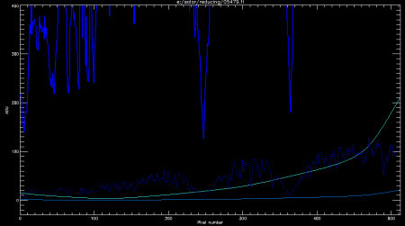
Fig. 3. The scattered light trace along the Ca HK order.
We present the same type of plot in Figure 3, showing the spline fit to the Ca HK order. This is a more straightforward task, since the order is straight and no ghost orders are present. Because of this we use a more widely spaced spline fit grid, with fits points placed near pseudocontinuum points along the HK order to ensure we capture all local scattered light.
In Figure 3, the Ca HK data are shown in blue (barely visible dipping into the top of the y-scaling) and in dotted blue (scaled down by a factor of 10, so that the whole spectrum is visible). The Calcium K and H lines are clearly apparent, centered at about pixels 245 and 365.
The thin blue line along the bottom of the plot shows the scattered light fit for this frame, as determined by the spline fit to the fit points. As expected for this single-order spectrum, it is quite low, but there is a gradual rise at the redward end of the order.
The light blue line shows the fit scaled up by a factor of 20. From this it is apparent the derived scattered light is ~1 ADU at Ca K and ~2-3 ADU at Ca H, rising to about 10 ADU at the red end of the order. The solid blue line shows that the Ca H and K line cores themselves lie at about 125 and 185 ADU, respectively, so as with the echelle, we obtain a scattered light background between about 0.5% and 1% of the data.
The final scattered light "surface"
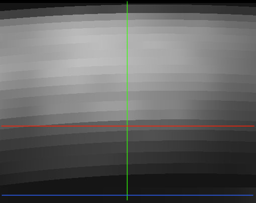
Fig. 4. The scattered light trace along the Ca HK order. The green, red, and blue lines show the x-axes of the plots in Figures 1, 2, and 3, respectively.
Figure 4 shows what our full scattered light image for the data frame above looks like. I have also added green, red, and blue lines that show the x-axes of the plots in Figures 1, 2, and 3. In particular, the red line shows why the scattered light background in Figure 2 appears to jump unphysically from one value to another; it's an artifact of the switch to a different order aperture along the CCD row.
The stripy look of the echelle section of the frame arises from our separate treatment of each order. The contrast of the grayscale is somewhat enhanced, and the grayscale undulations along each order represent variations of 1-5 ADU in the spline fit through the 50 points along each order. Regions at the very top and bottom of the echelle frame are black because we extract no data from these parts of the frame and set the scattered light in these areas to zero.
Long term trends in scattered light
It is important to monitor the data for any systematic trends in scattered light. Since this component is removed from the data frames before spectrum extraction, we do not expect it to have any impact on the final data, but it is nevertheless useful to be aware of trends in one's data.
In Figure 5, we present the ADU value of the background scattered light at pixel 245 along the dispersion axis of the blue HK order, which lies close to the core of the Ca K line. The long-term behavior of scattered light in the blue order is certainly one of the more interesting aspects of our data set.
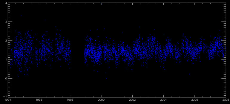
Fig. 5. The mean scattered light value, in ADU, near the core of the Ca K line. There is a very slight periodicity of about one year in the scattered light background.
As you can see in Figure 5, the scattered light background near Ca K has a clear periodicity of approximately one year. The effect is extremely small, with an amplitude of about 0.5 ADU, and thus will have a negligible impact on the Ca K time series, but it is clearly visible, with a higher background toward the middle of the year. The only explanation we have come up with so far is that this is an airmass effect; the Sun shines down more directly in the summer and we tend, on average, to have slightly less blue light scattered by the atmosphere and more going into our fiber. This is corroborated (though not necessarily proven) by the analogous data from the echelle, which do not show a similar periodicity (Figure 6).
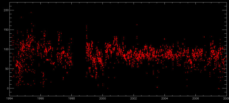
Fig. 6. The mean scattered light value, in ADU, near the center of the echelle frame. No significant trend is observed. The scatter in the data is indicative more of varying exposure depths than pathological CCD behavior.
An encouraging aspect of Figures 5 and 6 is the lack of any secular drift in the scattered light. Beyond the scatter in the light level on any given exposure due to the varying overall depth of the exposures, we observe no long-term drifts in the background behavior of either CCD.
Continue to a description of spectrum extraction.

[Back to contents]
[ Back to my home page | Email me: jch [at] lowell [dot] edu ]
The SSS is publicly funded. Unless explicitly noted otherwise, everything on this site is in the public domain.
If you use or quote our results or images, we appreciate an acknowledgment.
This site is best viewed with Mozilla Firefox.