The Solar-Stellar Spectrograph
[ Home | About | Tech Info & Data | Publications | References ] [ Site by Jeffrey Hall | Research funded by NSF ]
Ca II H&K stellar time series
At last the rubber meets the road! We have described in gruesome detail how we extract the spectra from the raw CCD frames, and how we place the Ca II H&K spectra on an absolute intensity scale. In this article, we describe (in technical terms) how we produce the time series plots of activity in the various stars on our program. The data products of this step are some of the fundamental results that come from our program, revealing the long-term activity changes in the Sun and Sun-like stars.
IDL procedure
We have one IDL method belonging to the OIL SSS class, SSS::stellar_hkseries, which analyzes the H and K spectrum stacks, writes the output text files to a results directory, and generates plots of everything we've done. It's 575-line monstrosity of a method, but most of it just involves setting up variables and generating plots. In this article, we describe exactly how the routine works, and how it determines the seasonal mean activity levels for our targets.
Output quantities
For broadest comparison with other programs, we calculate solar and stellar activity in four ways.
1. H and K indices. The raw H and K indices are just the residual intensities with in 1Å bandpasses centered on the cores of the H and K lines. These are directly comparable to the solar indices from the NSO data series, and have units of mÅ. A typical disk-integrated solar K index near activity minimum is ~87 mÅ.
2. Mount Wilson S. We calculate S from our HK indices via the general prescription given by
Hall & Lockwood (1995),


"The Solar-Stellar Spectrograph: Project Description, Data Calibration, and Initial Results." ApJ, 438, 404. [The first major paper from the SSS project.] except that we are using an empirical flux scale based on b-y rather than B-V (see
Hall 1996


"On the Determination of Empirical Stellar Flux Scales." 1996, 108, 313. [Measuring the continuum fluxes of stars in important bandpasses as functions of broadband colors.] for details). In addition, we can compute S directly from the spectra as a consistency check, since our HK coverage includes both the line core and reference bandpasses of the Mt. Wilson HKP instruments.
We calculate S via the standard formula
,
as described by
Duncan et al. (1991).


"Ca II H and K measurements made at Mount Wilson Observatory, 1966-1983." ApJS, 76, 383. [Contains a truly enormous table of activity measurements at Mount Wilson, plus a decription of the observing and reduction procedure.]
3. R'(HK). The R' index attempts to correct a color term in S arising from its dependence on the local continuum flux, and it is widely used in the literature (despite a few problems of its own). We use the formulation of
Noyes et al. (1984).


"Rotation, Convection, and Magnetic Activity in Lower Main-Sequence Stars." ApJ, 279, 763. [An important paper discussing the dependence of stellar activity on rotation and spectral type. Includes a widely used formulation of the R' activity parameter.]
4. The excess magnetic flux ΔF. We calculate this quantity via the method we developed in
Hall, Lockwood, & Skiff (2007).


"The Activity and Variability of the Sun and Sun-like Stars. I. Synoptic Ca II H and K Observations." AJ, 133, 862. [A summary of our calcium HK observations.] The idea is to isolate only that portion of the light in the HK indices arising from dynamo-related magnetic activity. This quantity is expressed in physical units (ergs cm^-2 s^-1).
For each of these quantities, we calculate grand means as well as seasonal means. The sections below outline how our routine does this.
Procedure
Step 1: Setting up the data
As described in detail in this article, the final product of our H and K data reduction is a set of four files that contain a stack of all observations of the MWO S bandpasses for a given star. These include the 20Å reference bandpasses and 6Å rectangles centered on the line cores. The 6Å widths are chosen to allow us to extract our 1Å rectangles as well as the 1.09Å FWHM triangles of the MWO photometers, and also to encompass enough of the inner line wings that we can inspect the time series for systematic drifts in the intensities (which turn out to be present in the old camera data, see below).

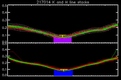
Fig. 1. A typical H and K line stack, in this case for the star 51 Pegasi (HD 217014).

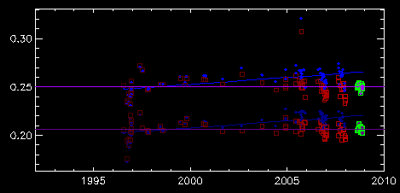
Fig. 2. H and K line wing trends for 51 Peg. Blue diamonds are the old camera data, red squares are the old data corrected for a systematic rise in line wing intensity of 0.01 between 1995 and 2008.
Figure 1 shows a typical line stack, in this case about 100 spectra of the star HD 217014 (51 Peg); K is at top, H at bottom. The pink and blue rectangles show the 1Å bandpass from which we make all our calculations; it is clear that the spectrum alignment and velocity-zeroing procedures of our reduction methods work well. Green spectra are those obtained with our new cameras in 2008 and beyond; red spectra are obtained with the old cameras. As always, the CCD improvement with the new equipment is obvious.
Two pairs of dotted lines are plotted with the K stack. These show the loci of 2σ and 4σ deviations from the mean line profile of all our observations. In determining seasonal means, we ignore all spectra where the inner wings deviate from the mean by more than 3σ.
Step 2: Examining and correcting line wing drifts
Examination of the 21,000+ spectra in the time series of our old camera data reveals a very slow increase in mean line wing intensity over time for all stars. The origin of this drift is unclear, but it is definitely an instrumental systematic not related to stellar activity. Measurements of the mean intensities in the absolutely scaled spectra at +/- 3 Å from the H and K line centers (i.e., near the edges of the plots in Figure 1) generally show an increase of approximately 0.01 between 1995 and 2008. This can be seen clearly in Figure 2, which presents the H (top) and K (bottom) line wing intensity measurements for 51 Peg. The straight purple lines show the mean intensity of the line wings for the new camera data (green squares). The blue lines are linear fits to the line wings of the old data (blue diamonds) and the red squares show the old camera data detrended by this fit.
This adjustment to the spectra is just the kind of thing to give one chills, since it alters the measured HK indices. We find this correction to be justified for three reasons.
1. All our stellar time series show this drift.
2. The drift is always in the same sense (increasing), and its magnitude is about the same for all stars.
3. The line wings in the early years of regular use of the old CCDs (1994-1997) are indistinguishable from those measured by the new CCDs (i.e., in terms of Figure 2, the linear fits in blue always cross the pink lines showing the mean new camera profiles in that time frame).
Therefore, we scale the H and K spectra in the line stacks to the mean wing profiles of the new camera data by dividing them by the difference between the new camera mean profile and the fit. The effect is shown in Figure 2; the blue diamonds are adjusted downward to the intensities shown by the red squares. These adjusted data are what is plotted in Figure 1.
We will document the effect of this procedure on the overall target set in another article. For now, we note that:
1. This is the only part of our stellar HK series routine that makes any change to the reduced data in the stacks; and
2. The changes introduced in S and other indices are well below the amplitude of typical stellar variability. We will have to examine this adjustment carefully only in the context of the flat-activity stars.
Computation of time series

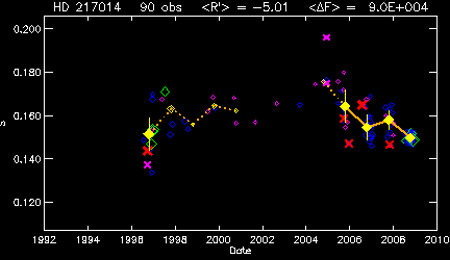
Fig. 3. The HK time series for the star HD 217014 (51 Peg), as of the end of 2008.
The remainder of our HK series routine calculates all the necessary quantities, stores the results in various output files, and creates a standardized plot of the HK data. One such plot is shown in Figure 3, giving S as a function of time.
Our routine automatically discards bad spectra using two criteria. If the line winds (after detrending as per above) deviate from the mean line profile by more then 3σ, the spectrum is not included in computation of seasonal means (these are marked with red X's in Figure 3). The thicker the X, the more deviant the spectrum. Likewise, very noisy spectra (S/N < 20) are not used (these are marked with pink X's). The spectra that survive our quality control methods (in Figure 3, 90 out of 98 observations made the cut) are used to compute seasonal mean activity levels in terms of the various indices.
In our standard plot at right, individual observations are shown by open diamonds. Green, blue, and pink symbols show progressively lower S/N spectra; the plot symbol size is also proportional to S/N. Yellow filled diamonds are the seasonal means, and the error bars show the standard deviation of the sample for that season. (The deviation of the means is estimated in the standard way, as the sample mean divided by the square root of the sample size.) "Good" seasons (which we somewhat arbitrarily define as those with >= 4 high-quality observations are marked with filled yellow diamonds and solid orange lines. Seasons with only 2-3 observations have open yellow diamonds and dotted lines to indicate the lower confidence in those trends.
The grand mean R' and ΔF are shown at the top of the plot.
Conclusion
The purpose of the time series generator routine described in this article is to produce data files with the HK measurements, as well as Figure 3, which provides a snapshot of the entire data set for a given star. In subsequent articles, we will discuss the results for all stars for which we have already published results in the peer-reviewed literature.
[Back to contents]
[ Back to my home page | Email me: jch [at] lowell [dot] edu ]
The SSS is publicly funded. Unless explicitly noted otherwise, everything on this site is in the public domain.
If you use or quote our results or images, we appreciate an acknowledgment.
This site is best viewed with Mozilla Firefox.