The Solar-Stellar Spectrograph

[ Home | About | Tech Info & Data | Publications | References ]      [ Site by Jeffrey Hall | Research funded by NSF ]

Ca II H&K solar time series

In another article, we have documented how we produce the H and K time series for the stars on our program. In this article, we describe the analogous procedure for our solar data. It is identical to the stellar procedure (as it ought to be) in all material respects.

IDL procedure

We use an SSS class method, SSS::solar_hkseries, to produce our solar HK series. It is quite analogous to the stellar routine. We are able to simplify it somewhat, since we do not need to compute various quantities based on the input star color but can rather just use the known (or at least adopted) solar values. The method calculates the same activity quantities we determine for the stars (HK indices, S, R', and ΔF.).

When we do a solar observation, we typically take a set of flat fields and three different solar exposures; we also occasionally do a Thorium-Argon spectrum to monitor the evolution (if any) of the wavelength solution. These four or five frames constitute a "day" of solar observations. Our solar HK series routine generates the output quantities above for each solar observation, and then calculates (1) the mean of the observations for a given day, which we use as the basic datum for that day, (2) "seasonal" (i.e., yearly) means, and (3) the grand mean; the latter two are for comparison with the analogous stellar quantities.

Procedure

Step 1: Setting up the data

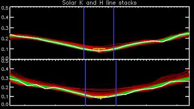
Fig. 1. The solar H and K line stacks, 1994-2008. The Kurucz solar spectrum at the resolution of the SSS is shown in white. Pre-2008 data (old cameras) are in red, while 2008+ data (new cameras) are in green. Over 4,100 solar spectra are overplotted in this figure. A few bad spectra are apparent as obviosuly discrepant line cores; these are flagged by the solar_hkseries routine and are not used in the results.

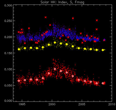
Fig. 2. The solar HK time series, 1994-2008, shown in terms of the HK index (blue), Mount Wilson S (yellow), and ΔF. (red). See text for discussion of scaling and generation of the data.

Our routine first extracts the H and K order from all the normalized solar spectra in our archive and assembles them into a huge array akin to the spectrum stacks we use for the stellar time series. As of December 2008, this encompasses roughly 4,100 observations obtained on 1,303 different days.

We then shift the spectra in wavelength so that they lie at zero velocity, and we check the line wings for systematic discrepancies. This is exactly analogous to the stellar procedure, except that in examining the line wings we use the Kurucz high-resolution solar spectrum degraded to the resolution of the SSS as the reference. The resulting stacks for the K and H lines for more than 4,100 spectra are shown in the upper and lower panels of Figure 1, with the Kurucz spectrum at the resolution of the SSS overplotted in white.

Interestingly, the gradual rise in line wing intensities observed in the stellar data (see the stellar HK time series article for details) is not observed in the solar data. There are two essential differences in the solar versus stellar observations: (1) the optical path is different (the solar observations bypass the 42" telescope) and (2) the observation lengths are different (~1-2 seconds for solar observations versus 10-20 minutes for stellar observations with the old cameras). While there is of course some scatter of the solar data about the reference spectrum, there is no secular trend and the data are generally scattered about unity relative to the Kurucz data.

Step 2: Generating the results

We calculate the four output quantities in exactly the same way we do for any of our stellar targets. The fundamental datum is the 1Å HK index. The rectangular bandpass for the K and H lines is shown by the vertical blue lines in Figure 1. The results are shown by the blue data points in Figure 2; for these data, the y-axis of Figure 2 has units of Å. Individual observations are faintly visible as red dots, while the small blue diamonds are the daily means. As with the stellar time series, red X's indicate data that we delete due to large (> 3σ from the Kurucz profile) discrepancies in the line wing intensities. Large filled diamonds show the yearly means for each quantity plotted

Our solar Mount Wilson S results are shown by the yellow data in Figure 2; in this case, the y-axis is S itself. Our results are in extremely good accord with the MWO solar series published by Baliunas et al. (1995).     
"Chromospheric Variations in Main-Sequence Stars. II.." ApJ, 438, 269. [The second "fundamental results" paper from the Mt. Wilson project, following Wilson (1978). Written for professional audiences but a classic.] This is encouraging since we plot here our derived S values (i.e., calculated from the flux inferred from the HK indices via our empirical flux scales, and the conversion technique given by Middelkoop (1982)     
"Magnetic Structure in Cool Stars. IV - Rotation and Ca II H and K Emission of Main-Sequence Stars." A&A, 107, 31. [Presents a method for converting fluxes to Mount Wilson S.] and Rutten (1984).     
"Magnetic Structure in Cool Stars. VII. Absolute Surface Flux in Ca II H and K Line Cores." A&A, 130, 353. [Extends the Middelkoop (1982) flux-S conversion. We (Hall & Lockwood 1995) have argued that the solar calibration in this paper is in error.] (To generate the solar indices, we use our own conversion constant that corrects what we (Hall & Lockwood 1995)     
"The Solar-Stellar Spectrograph: Project Description, Data Calibration, and Initial Results." ApJ, 438, 404. [The first major paper from the SSS project.] have argued is an error in Rutten's paper.) We find a mean S of ~0.170 for the relatively weak solar cycle 23.

Finally, our excess magnetic flux values ΔF are shown in red. The units here are ergs cm^-2 s^-1, and the data have been scaled own by a factor of 4 x 10⁶.

All these quantities are directly related, of course, so the overall character of Cycle 23 is the same for any of them. Since this article is more about the generation of the results than an analysis of them, we note here that our most recent data (following the hole in the dataset in 2008 while we replaced our cameras) do seem to show the bottoming out of Cycle 23 after its rather majestic decline. We also do see (albeit somewhat weakly) the double-peaked nature of Cycle 23, with periods of very high activity in later 2000 and in 2002.

[Back to contents]