Composite Spectral Indices: A New Method
for the Interpretation of Activity in the Sun and Solar Analogs
Jeffrey C. Hall
Lowell Observatory, 1400 W Mars Hill Rd, Flagstaff, AZ, 86001
jch@lowell.edu
1. Introduction
Discussions of the behavior of the H and K lines of singly ionized calcium
in large samples of cool stars span the modern literature (e.g., Wilson & Bappu 1957,
Baliunas et al. 1995). The long- and short-term behavior of these lines,
which serve as proxies for chromospheric activity, has revealed direct observational
evidence for stellar activity cycles, rotational modulation, and even differential
rotation. As this workshop has demonstrated, however, it has been very difficult
to properly evaluate the Sun as a star, and almost impossible to agree on what star
is most nearly solar-like.
2. Origin of the problem
- [1] It is difficult to observe the Sun in exactly the same way that we observe the
stars.
- [2] Detailed, high-resolution spectral studies (leading to precise determination of
fundamental parameters, e.g., Teff) preclude large, synoptic surveys (leading to a knowledge
of the behavior of the general stellar ensemble), and vice versa.
- [3] The only very long-term, synoptic database of stellar activity (the 30-year time series from Mt. Wilson)
is limited to one spectral feature, and while the contribution of these data to our
understanding of stellar activity has been enormous, we know that a star that is a solar
twin in terms of parameter X may look decidely un-solar in terms of parameter Y.
- [4] Identifying solar analogs in terms of variability is of critical importance,
considering the present evidence that solar irradiance variations may profoundly affect
terrestrial climate. But the link between chromospheric variability and total irradiance
variability is tenuous, although Lockwood, Skiff, & Radick (1997) have presented a
large observational database addressing this issue, and inferring irradiance variations
from Ca II data is not possible at present.
3. Approaches to solving this problem
Our Solar-Stellar Spectrograph (S3) program (see, e.g., Hall & Lockwood 1995) offers
a method of addressing issues [1] through [3] above.
- Re [1]: We transmit starlight and unresolved
solar light through optical fibers to the same spectrograph, obviating inter-instrument
calibration difficulties and coming as close to true ``Sun-as-a-star'' observing as the
diurnal atmospheric variability permits.
- Re [2]: The S3 has an echelle spectrograph spanning the wavelength range 5100-9000
with 70% coverage, and a Littrow spectrograph spanning the wavelength range 3860-4010
(Ca H&K). The resolution is 12,000 for the echelle, and slightly
lower for the Littrow, which does not directly solve the central problem of issue [2]
above. But, see next section.
- Re [3]: Instead of one spectral feature, we observe well over 200, including
all the classic chromospheric diagnostics. These spectral features cover atomic species
with a wide range of characteristics (e.g., equivalent width, excitation potential,
depth of formation). With approximately 7800 data frames at our disposal, we have
about 1.6 million measurements of spectral features in the Sun and hundreds of
solar-like stars at our disposal.
- Re [4]: But, says the skeptic in us, we know the total solar irradiance (TSI)
variability is under 1%; how can we hope to identify variability in inactive, solar-like stars,
especially given our typical signal-to-noise of 50-100?
4. The Solar Rotation in SSS Data
4.1. Periodogram analysis of solar data
We calculated the Scargle periodogram (as presented by Horne & Baliunas 1986)
of our solar Ca II K data set. This comprised
observations on about 300 days between the beginning of 1994 and late 1997. Although
we observed power in the periodogram at the 27-day rotation period of the Sun, it was
not significantly above the multitude of noise spikes typically present in such
analyses. But, then we did the following:
- [1] We calculated periodograms for 120 lines in the solar spectrum.
- [2] We filtered out the strongest peak in each of these periodograms with
omega gt 0.01 d-1.
- [3] We recalculated the periodogram with this one dominant frequency now removed.
- [4] We averaged the resulting set of periodograms.
The results of this procedure are shown in the figures. In the following figures, we show the
results obtained from this procedure. These figures are similar to the
figure published by Hall & Lockwood (1998), but they incorporate additional solar data
from the end of 1997.
The greyscale image in the bottom part each figure shows the 120 periodograms stacked
vertically. No attempt to identify specific spectral lines is made; they are simply
numbers 1-120. The greyscale bar in the central part of each plot is the average
of the 120 periodograms, and at the top of each is a graph of the average.
4.2. Raw periodogram analysis
We produced Figure 1 by using steps [1] and [4] of the above procedure only.
That is, we calculated the periodograms and averaged them.
There are prominent peaks in the power spectrum at 27.4, 13.7, and 9.13
days. These are the fundamental, 2:1, and 3:1 harmonics of the solar rotation
period, and they are identified by the dashed vertical lines. The centroids of these
peaks fall precisely at the harmonic frequencies (within 1%). At extreme left are
three very large peaks, identified by the solid line. The lowest-frequency peak
goes well off the vertical scale plot. These peaks lie at 355, 180, and 120 days,
and are the fundamental, 2:1 and 3:1 harmonics of the annual variation in the
telluric water vapor lines. (In Arizona, this is a pronounced yearly variation,
with the July-September monsoon producing a noticeable increase in water vapor
absorption across the entire SSS echelle spectrum.)
Also visible are several other prominent peaks, the most significant of which
lies at omega ~ 0.024 (41.6 d). The two other dotted lines in this
figure lie at 2:1 and 3:1 harmonics of this 41.6-day period. Although other
peaks exist in Figure 1, they do not coincide with these harmonics.
4.3. Filtered periodogram analysis
In Figure 2, we have added steps [2] and [3] above. For each of the
120 spectral lines, we calculated the periodogram, filtered out the strongest
period in the data less than 100 days, and recalculated the periodogram. We
then averaged them as before. The rationale here is that if the solar rotational
signal is comparable to or less than the noise, it will usually not be the
strongest peak in the spectrum. Thus the filter should preferentially remove
noise, and any surviving peaks arising from a real signal are likely to
be enhanced. We limited this filter to P less than 100 d because (1) this is the
regime of physical interest and (2) the telluric signals dominate the
P greater than 100 d area.
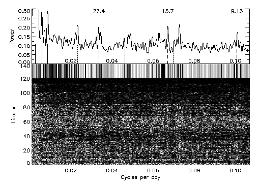
FIGURE 1:The
averaged periodogram of 120 spot-sensitive lines in the solar spectrum.
The greyscale image at bottom shows the stacked individual periodograms, while the greyscale
bar and the graph above it are the average of these 120 periodograms.
A series of peaks, at 27.4 days and at 2X and 3X harmonics of this period, is apparent.
These correspond to the solar rotation period. A 355-day telluric peak and its 2X and 3X
harmonics are also apparent (solid lines at left). None of the other peaks in the
spectrum are harmonically related. Note that the x-axis of this scale is a synodic
frequency scale, while the labeled peaks have been corrected to the sidereal period
corresponding to the solar rotation.

FIGURE 2:This is
the same plot as Figure 1, except that in each individual periodogram,
we have filtered the strongest peak with frequency omega gt 0.01 cyc d-1. The
solid, dashed, and dotted lines are in the same locations as in Figure 1. The harmonics
of the solar signal are gone, as is the strong peak around 0.024 cyc d-1. A
weak, high-frequency signal has appeared around 0.095 cyc d-1, but it is
insignificantly above the other weak peaks scattered through the spectrum. The telluric
peaks are unaffected by the filtering, as they lie outside the frequency region subjected
to it. The only significant feature lying in the physically significant frequency region (as
far as stellar rotation is concerned) is at 27.4 days.
We have left all the solid, dashed, and dotted lines from Figure 1 unchanged
in Figure 2, to allow easy comparison of the location of the peaks from
figure to figure. The essential result in
Figure 2 is that the only peak that survives the
filtering procedure discussed above is the 27.4-day peak. The other
pronounced peaks apparent in Figure 1 are gone, as are the harmonics of
the posited solar signal. We believe the 27.4-day peak arises from a real
signal in the data, therefore, for two reasons:
- In Figure 1, we know the telluric peaks are real, and they show perfectly-spaced
2:1 and 3:1 harmonics. The 27.4-day peak shows identical harmonics, while none of
the other significant peaks in Figure 1 show any harmonic relationships.
- In Figure 2, application of a procedure that preferentially removes noise
gets rid of all the peaks except one, at 27.4 days.
It seems quite likely that we have detected the solar rotation at solar minimum,
with resolution 12,000 data of S/N ranging from 50 to 150.
5. Composite Spectral Indices
Athay & White (1992) found, in an examination of early SSS data, ``no rotational
modulation of the solar irradiance spectrum at either H alpha or Ca II.'' We did
not, either, using the individual spectral indices examined by Athay & White.
But in the previous section, we have created what we term a Composite Spectral
Index (CSI) of solar irradiance data. We can measure over 200 lines in our SSS
solar data; for Figures 1 and 2 we have used only the 120 that Moore et al. (1966)
classifies as either strongly or weakly affected by the presence of sunspots. Figure
1 and Figure 2 therefore result from a subset of our data that we expect to be
(a) related and (b) indicative of solar activity. This leads us to the basic
definition of this paper:
A composite spectral index is an indicator of
solar and stellar activity produced by combining time-series data for some
number N of spectral lines that are related in terms of properties (p1, ... , n).
Although the idea of the CSIs came to us as a result of the periodogram analysis,
we will not, in general, define our CSIs in this way.
Periodogram analysis of our stellar targets, as we have done for the Sun, will be difficult for
some targets and impossible for most, because the data sets are much smaller.
However, examination of the flux variability in sets of lines with different characteristics is
more encouraging. The variability in spot-sensitive sets of lines in our solar data, both
on yearly and monthly timescales, is significantly greater than that in spot-insensitive
lines. The same holds for our 18 Sco data set. It therefore seems that CSIs, particularly
those based on physical properties of the lines in question (e.g., excitation potential),
can serve as new indicators of solar and stellar activity that are closely tied to the
physical processes at work in the atmospheres. We are still in the stage of developing
different CSIs and testing them on our data as of this writing, so no results in this
direction are presented here.
The essential difference between this approach and that of
extant long-term studies is the use of many
related spectral features to uncover signals in the data that are hidden in
individual features by noise. The broad-based
nature of a well-chosen CSI may make it a more physically significant indicator
of the mechanisms producing solar and stellar variability than an indicator based
on a single line. Additionally, we can compare the Sun with individual
stars in this way, rather than with snapshots of the stellar ensemble. This is
a basic shift in our analysis paradigm for our SSS data. Instead of studying
``the Sun as a star,'' we will now be examining in detail the myriad features in our
spectra of solar analogs, to study ``the stars as a Sun.''
6. Conclusion
More or less by accident, we discovered that we can detect the solar rotation in
moderate-resolution, moderate- to good-quality solar spectra with approximately
4-day time resolution, at solar minimum. The decision to run 200 periodograms on
supposedly ``boring'' spectral lines was more of a ``let the workstation run all night
and see what it coughs up'' decision than a burst of physical insight. Yet we now
have a potential avenue for an exhaustive investigation of our 10,000 solar and
stellar data frames. The 20 spectral order in an SSS data frame span 5,120 CCD pixels.
By studying just the traditional Ca II H & K, Halpha, and the Ca II IRT lines,
we were using about 10 of those pixels. We are now examining the content of
our data in detail, to sort the spectral features we observe into meaningful classes,
and to derive information about solar and stellar variability from them. Our hope is
that examination of variability in a large number of lines formed throughout the
photosphere, rather than just the chromosphere, will allow us to tie our spectroscopic
data to broadband irradiance variations from other programs (e.g., Lockwood, Skiff,
& Radick 1997). Results of these investigations will be forthcoming in the literature
over the next few years.
References
Athay, R. G., & White, O. R. 1992, NCAR Technical Note (NCAR/TN-375+1A).
Baliunas, S. L., et al. 1995, ApJ, 438, 269.
Hall, J. C., & Lockwood, G. W. 1998, ApJ, 493, 494.
Hall, J. C., & Lockwood, G. W. 1995, ApJ, 404, 416.
Horne, J. H., & Baliunas, S. L. 1986, ApJ, 302, 757.
Lockwood, G. W., Skiff, B. A., & Radick, R. R. 1997, ApJ, 485, 789.
Moore, C., et al. 1996, The Solar Spectrum 2935 A to 8070 A
(Washington: National Bureau of Standards).
Wilson, O. C., & Bappu, M. K. V. 1957, ApJ, 125, 661.
[Contents]